Electrical Waves and Impedance Matching
Aditya Mittal
Experimental Physics II
(PHY462)
Lab Report
Monday, May 07, 2007
Introduction:
Electromagnetic waves travel through any given
medium. However, their propagation is “characterized
by the impedance of the particular medium” [1], and at the interface of two
such media a traveling electromagnetic wave can be partially or fully
transmitted or reflected depending upon the relative impedances of the two
media.
A transmission line is an entity through which an
electromagnetic wave is propagated.
Examples of transmission lines include twisted pairs, coaxial cables,
waveguides, microstrips etc. In this experiment we will be using BNC
cables (coaxial) and microstrips. The transmission lines have characteristic
impedance, and for these common types of transmission lines, the formulae used
to determine the characteristic impedances have been previously determined for
us. We will not be deriving them from
Maxwell’s equations, according to prof. Plourde.
In our experiment we explore terminating the
transmission lines with some characteristic impedance. This termination or load impedance might be
different from that of the transmission line and allows us to explore the
reflection and transmission of the electromagnetic waves. When the terminating impedance is equal to
the impedance of the transmission line, known as impedance matched circuit, we
get full transmission.
When the terminating impedance is an open circuit, we
get an equal amplitude pulse to reflect back, and when the terminating
impedance is a closed circuit, we get a pulse of negative the amplitude of the
original pulse back. This reflection is
characterized by the coefficient Г = (Z2 – Z1) / (Z2 + Z1) where Z2 is
the terminating impedance and Z1 is the impedance of the transmission line. “Г is a complex quantity relating the
amplitude and phase of the reflected wave.” [1]
For most of the real applications, the idea is to
make the impedances Z2 and Z1 equal so that the full wave is transmitted. Otherwise, we would get power loss, which is
something we don’t generally want.
Often, radio and fiber optic cables are treated as transmission lines,
and in these we want the full signal to be transmitted, and don’t desire signal
loss.
Experimental Technique:
Apparatus
1. Agilent arbitrary waveform generator, 33250A
2. Digital oscilloscope – the 2-channel Instek scopes are sufficient
3. Mini-circuits power splitter, ZFRSC-42
4. BNC-SMA adapters, BNC cables (several lengths), 50
Ohm terminators
5. Circuit board pieces and SMA connectors for microstrip fabrication
6. Additional inductors (.47uH), capacitors (1nF),
and resistors (68, 47, 220, 23.5Ω)
7. Soldering Station for Soldering different LRC
Circuits together for terminators
8. Shorting Cap
Schematic
Measurement Procedure
We began by investigating the arbitrary waveform
generator outputting narrow and wide pulses at different frequencies by
connecting its output directly to a channel on the oscilloscope. We checked out amplitude, pulse height,
width, edge time, and frequency setting.
We also used the sync signal as the external trigger to the
oscilloscope.
The real connections are shown in the schematic
above. The transmission Line and
Terminating Impedance are the Load and can have resistive, capacitive, or
inductive components.
Then in this experiment we used a pulse propagation
technique to measure the velocity of wave propagation along a coaxial cable. This technique involved sending a pulse
through a coaxial cable, and then measuring the time it took to get the
reflected wave back from the original wave.
By dividing the distance with the time it took to get the wave back we
could determine the propagation velocity of the electromagnetic wave.
Next, we do impedance matching with the 50 Ohm
Terminator end on Channel1 of the Oscilloscope, and adding a 50 Ohm termination
as the load at the end of the power splitter.
This results in no reflected wave.
Second part of the measurement process just involved
setting up different terminating impedances using various LRC combinations and
looking at the various resulting reflected waves on the Oscilloscope from the
mismatch interface.
Finally, we fabricated a microstrip
line by cutting out the copper on the circuit board pieces with a razor to
produce a microstrip line. We soldered SMA launchers onto either end of
the board so we can connect to the microstrip line.
We made our microstrip line
have an impedance of 20 Ohms, and observed its behavior as a transmission line
using the previous process.
Difficulties and Anomalies
When I was working with
Prof. Plourde on looking at the microstrip
waveforms from using multiple BNC cables, we encountered some odd waveforms
because there was transmission at the interface between the BNC cables. We believe that was because of the BNC cable
that was picked up from somewhere else being of different impedance or
something wrong going on with it.
Mostly, things seemed to be as expected at the
various interfaces. We did not have much
trouble with matched impedance to begin with.
It took me a while to understand how both the cursors work with one
button on the weird oscilloscope.
Reporting and Analyzing Data
Delay Time versus Cable Length to figure out Propagation Velocity
|
Delay
time (ns) |
Two
times of cable lengths (cm) |
|
11.3 |
228±9 |
|
21.6 |
420±9 |
|
27.9 |
550±9 |
|
36.6 |
740±9 |
|
48.2 |
964±9 |
Since the wave goes back and forth, we double the
cable length as the distance traveled and we have our delay time so we can now
determine the propagation velocity. The
reason we used ±9 cm for our error is because
the BNC cables were of length 4.5cm. The
slope of the graph gives us the propagation velocity as 20.2 cm/ns = 20.2 x 10⁸
m/s.
I am not sure about this number, I thought it should
have been 50 Ohms, as we are using cables that are either BNC-C-60 or RG58A/U or
POMONA 2249-C-36 (RG 58C/U) and according to http://www.tequipment.net/PomonaBNC-C.asp
and http://www.tessco.com/products/displayProductInfo.do?sku=96931&eventPage=1
and http://www.rapid-tech.com.au/Pomona.htm
they should all be 50 Ohms.
Various LRC Terminators
50 Ohm terminator
We don’t see any reflected
wave i.e. we just see the original wave with no attenuation. This is of course, what we expected based on
Г = (Z2 – Z1) / (Z2 + Z1) since now both Z2 and Z1 are 50 Ohms. The original pulse wave varied from 0V to
2.45V, so that is what we got back. The
wave we expect to see is the original wave superimposed with the reflected
wave, and since there is no reflected wave, we just see the original wave. The reflected wave will be equal to Г *
Original wave, and in this case Г = 0.
Open Circuit
In this case Г = 1 as
Z2 approaches infinity and we can apply L’Hopital
Rule to see that Г approaches 1.
This causes the full wave to be reflected back, which makes sense in
that electromagnetic waves do not travel in empty space. Of course, our open circuit terminating
impedance is air and so the impedance is not going to be infinity. On the oscilloscope we measured the wave to
be from 1.11V to 2.45V.
This gives us that the
amount of wave reflected back is 2*1.11/2.45 = 91%. From this we can use Г = (Z2 – Z1) /
(Z2 + Z1) to solve for Z2 when Г = .91 and Z1 = 50. We get Z2 = 1013 Ohms. This makes sense as it is high impedance,
which is what we expect of an open circuit.
Zero Impedance Circuit
In this case Г = -1 as
Z2 = 0 and we get Г = -50/50. This
causes the full wave to be reflected back with negative amplitude, which makes
sense in that electromagnetic waves could not escape the transmission line
since the circuit was closed. Of course,
our closed circuit terminating impedance is a shorting cap which may have a
small resistance of its own. On the
oscilloscope we measured the wave to be from 1.21V to 2.45V.
This gives us that the
amount of wave reflected back is 2*-1.21/2.45 = -99%. From this we can use Г = (Z2 – Z1) /
(Z2 + Z1) to solve for Z2 when Г = .99 and Z1 = 50. We get Z2 = 0.25 Ohms. This makes sense as it is very small impedance,
which is what we expect of zero terminating impedance circuit.
68, 220, and 23.5 Ohm Resistances
Similar idea, we measured
the wave and calculate the amount reflected back and use that to determine Z2.
|
Resistance (Ohms) |
Reflection coef. |
Calculated Z2 |
% Error |
|
68 |
2(0.19/2.45) = 0.16 |
69 Ohms |
.015 |
|
220 |
2(0.78/2.45) = 0.64 |
228 Ohms |
.036 |
|
23.5 |
2(-0.50/2.45) = -0.41 |
20.9 Ohms |
.111 |
The error in all three cases
is small, so that’s good.
1nF Capacitance

In this case we are
reading the voltage on the oscilloscope for various delay times with the
Capacitance of 1nF. The error in voltage
is from our ability to read the oscilloscope.
From this we can make the following voltage versus delay time graph:
From the graph we get the
value of tau to be 47.7 ns and we use this value to
calculate the capacitance. As we know
from introductory courses in electronics tau is the L/RC
constant and we have no inductor and so to get C all we need to do is divide
the tau by the resistance of 50 Ohms in this
case. C = 47.7ns / 50 Ohms gives a
capacitance of 0.95nF, which is pretty close to the actual value of the
capacitor of 1nF.
We can also look at
propagating the error in this case.
Measuring the resistance of the 50 Ohm terminator directly, we measured
52.8 Ohms and so the terminator has at least an error of ±2.8 Ohms. The error in the value of Tau
is given by Origin to be 3.68 and so adding the fractional errors to get the
fractional uncertainty in Capacitance we get 0.133. Multiplying this by our measured value we get
0.130 x 10⁻⁹ F.
So, our value is C = 0.95nF
± 0.130nF. 1nF is within this acceptable
range.
.47μH Inductance
Just like for capacitance,
we again measure voltage versus delay time using the scope and graph it.
|
Delay time (ns) |
Voltage (V) |
error value of voltage (V) |
|
0 |
1.94 |
±0.03 |
|
4 |
1.31 |
±0.03 |
|
8 |
0.89 |
±0.03 |
|
12 |
0.54 |
±0.03 |
|
16 |
0.39 |
±0.03 |
|
20 |
0.24 |
±0.03 |
|
24 |
0.15 |
±0.03 |
|
28 |
0.13 |
±0.03 |
|
32 |
0.08 |
±0.03 |
|
36 |
0.06 |
±0.03 |
|
40 |
0.04 |
±0.03 |
|
44 |
0 |
±0.03 |
|
48 |
0 |
±0.03 |

This time we don’t have a
capacitor but an inductor so tau = L/R, where L is of
course the inductance. So L = R*tau = 50 Ohms * 9.90ns = 0.5μH.
We can calculate the error
again by using the fractional error = (2.8/50) + (0.23/9.90) = 0.079. Multiplying by 0.5μH we get
.04μH. Indeed, 0.47μH is
within .5μH ± 0.04μH.
Microstrip Line
 http://wcalc.sourceforge.net/microstrip.png
Using
equation 1.20 from Microstrip Lines and Slotlines by K.C. Gupta, Ramesh
Garg, and I.J. Bahl, we
first calculated with Maple software the desired width of the strip for
creating a 20 Ohm microstrip. The equation is the following:
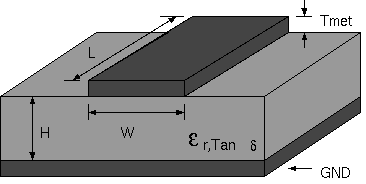
Here, h is the height of the microstrip
and in our case it is known to be 1.45 x 10⁻³ m. Also, on the lab table the permittivity for
the dielectric is given to be ε = 2.94 ± 0.04 which has been substituted
in the above expression from the equation 1.20 of Guta,
Garg, and Bahl. We got the value for our desired strip width
to be 0.0127 from Maple for a 20 Ohm microstrip and
so we fabricated a microstrip line by cutting out the
copper on the circuit board pieces with a razor to produce a microstrip line and soldering SMA launchers onto either end
of the board so we can connect to the microstrip
line.
For quite some time we looked at the configuration
with different setting with prof. Plourde,
and eventually we measured the wave as going from -9.42V to 260V for the
particular impedance change between the BNC cable and the microstrip. We also analyzed the waveform to try to
understand what was happening at different boundaries with the microstrip and how that was affecting the reflected wave.
Again we calculated the percentage of reflected wave
as 2*-9.42/260 = -7.2% and then used it to get the Z2 = 43.3 Ohms.
Then we went ahead and tapered the tabs to make the microstrip look more like in order to reduce the affect of
capacitance on the impedance. This made
the oscilloscope value go from -7.8V to 260V resulting in a calculated Z2 of
44.3 Ohms. Not quite the 20 Ohms we were
looking for but it’s a complicated geometry and the equations and everything
are approximate and on top of that there are experimental errors.
Conclusion
Overall, we learnt quite a
lot about transmission lines and impedance matching in this lab. I wish we had more time then we could have
played some more with these things, but the semester flies by rather
quickly. Although, I have not discussed
all the readings here, they have also been fun and extremely instructive. Thanks to prof. Plourde for all his explanations because they are some of
the most enlightening ones. Now I’m
curious to go learn about the impedances of all kinds of things like waveguides
and many other geometries and substances etc.
References
[1] PHY462 Electrical Waves
and Impedance Matching Draft http://physics.syr.edu/courses/PHY344.07Spring/labs/impedance-match.pdf
[2]
Microstrip Lines and Slotlines by K.C. Gupta, Ramesh
Garg, and I.J. Bahl
[3]
Chapter 8, Impedance Measurement from Planar
Microwave Engineering : A Practical Guide to Theory,
Measurement, and Circuits by Thomas H. Lee of
[4]
http://www.williamson-labs.com/xmission.htm
[5]
http://en.wikipedia.org/wiki/Transmission_line
[6]
http://en.wikipedia.org/wiki/Coaxial_cable
[7]
ELE490 I learnt about waveguides and optical cables
in independent study under Prof. Kornreich.
[8]
Mathematical Analysis of Digital Systems I learnt
about transmission lines, attenuation, cross talk etc. in that course under
prof. Nunez.